CNC TAP File Visualizer

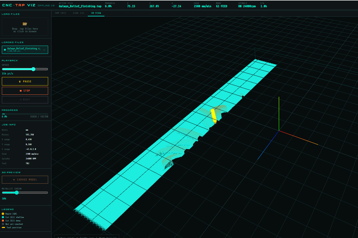
A browser-based visualizer for CNC .tap / .nc / .gcode files. Runs entirely offline — no server, no install. Drop a file in and watch the toolpath play back.

View on GitHub

What it does

  • Parses G0/G1 3-axis milling and G81 drill cycles
  • Animates the toolpath with adjustable playback speed (0.05 pt/s up to 5k pt/s)
  • Three views: Top (XY), Side (XZ), and a full 3D orbit view via Three.js
  • Colour-codes moves by depth — shallow cuts in cyan, deep cuts in orange, rapids in yellow
  • Builds a carved mesh from the toolpath so you can preview what the stock will look like after machining
  • Multi-file support with per-file colour assignment
  • Shows live X/Y/Z position, feed rate, spindle state, and ETA during playback

3D view

CNC TAP Visualizer - 3D view

The 3D view renders the full toolpath as line segments with depth-mapped colouring. Left-drag rotates, scroll zooms, right-drag pans.
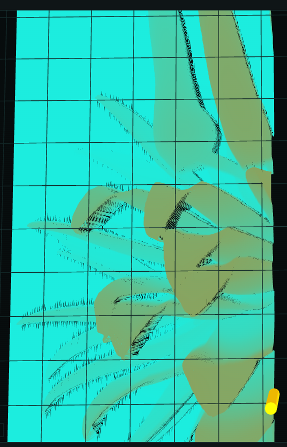
Carved model

CNC TAP Visualizer - carved mesh detail

The carved model is built by walking every toolpath segment and recording the minimum Z reached at each grid cell (120×120). The result is a height-mapped mesh showing which areas have been cut and how deep. Useful for catching missed regions or checking depth consistency before running the job.

G-code support

1
2
3
4
5
6
7
8
G0  — rapid positioning
G1 — linear feed move
G81 — canned drill cycle (with R-plane retract)
G80 — cancel canned cycle
G20 / G21 — inch / mm units
S — spindle speed
T — tool number
F — feed rate

Implementation notes

  • No build step. Single HTML file with an inline <script> block.
  • Three.js loaded from CDN (r128). Everything else is vanilla JS.
  • Large files (>80k points) are downsampled while preserving rapids, Z-direction changes, and the first point after every rapid. A 600k-point finishing file samples down to ~80k without losing the toolpath shape.
  • The carved mesh walks segments using a Bresenham-style interpolation so long roughing strips fill every grid cell between endpoints, not just their start and end.
  • Speed slider uses a log scale: slider position 1–1000 maps to 0.05–5000 pt/s.

Limits and Continuity Fundamentals

Limits are the foundation on which derivatives and integrals are built. A limit
describes the value a function approaches as its input approaches a point — the
function need not be defined at that point. Continuity asks whether the
function actually attains that value, or whether something fails at the point.

Definition of a limit

Consider:

$f(x) = (x^2 - 1) / (x - 1)$

At x = 1 the expression is undefined (0/0). Evaluating near x = 1 — at
x = 0.99, 0.999, 1.001, 1.01 — the outputs approach 2. The limit is 2,
even though f(1) does not exist.

Three standard approaches to evaluating a limit:

  • Graphically — inspect whether both sides converge to the same value.
  • Numerically — tabulate f(x) for inputs approaching a and observe the trend.
  • Algebraically — simplify using limit laws.
1
2
3
4
5
6
7
import numpy as np

x_vals = np.array([0.9, 0.99, 0.999, 1.001, 1.01, 1.1])
f_vals = (x_vals**2 - 1) / (x_vals - 1)

for x, y in zip(x_vals, f_vals):
print(f"x={x:.3f}, f(x)={y:.6f}")

Formal definition

$\lim_{x \to a} f(x) = L$ means f(x) can be made arbitrarily close to L by
taking x sufficiently close to a, without requiring x = a.

The epsilon-delta formulation makes this precise — see the worked proof below.

One-sided limits

  • $\lim_{x \to a^-} f(x)$ — the left-hand limit, approaching a from below.
  • $\lim_{x \to a^+} f(x)$ — the right-hand limit, approaching a from above.

The two-sided limit exists if and only if both one-sided limits exist and are equal.

Limit laws

When the individual limits exist, they obey the following rules:

  • Sum: $\lim(f+g) = \lim f + \lim g$
  • Difference: $\lim(f-g) = \lim f - \lim g$
  • Product: $\lim(fg) = (\lim f)(\lim g)$
  • Quotient: $\lim(f/g) = (\lim f)/(\lim g)$ — provided the denominator limit is nonzero
  • Power: $\lim(f^n) = (\lim f)^n$
  • Composition: if f is continuous at L, then $\lim f(g(x)) = f(\lim g(x))$

Indeterminate forms

Indeterminate forms such as $0/0$ or $\infty/\infty$ have no immediately
obvious value. Standard resolution techniques:

  • Factor and cancel
  • Multiply by the conjugate
  • Apply trigonometric identities
  • Use series expansions

Factor and cancel:

$\lim_{x \to 1} (x^2 - 1)/(x - 1)$

Since $x^2 - 1 = (x - 1)(x + 1)$, for $x \ne 1$ the expression reduces to $x + 1$.

$\lim_{x \to 1} x + 1 = 2$

Continuity

A function f is continuous at x = a if and only if:

  1. f(a) is defined
  2. $\lim_{x \to a} f(x)$ exists
  3. $\lim_{x \to a} f(x) = f(a)$

If any condition fails, f is discontinuous at a. Discontinuities are classified as:

  1. Removable — the limit exists, but the function value is absent or incorrect
  2. Jump — left and right limits are finite but unequal
  3. Infinite — the function diverges near the point
  4. Oscillating — the function does not converge to any value (e.g. $\sin(1/x)$ near 0)

Removable discontinuity

$f(x) = (x^2 - 1)/(x - 1)$ reduces to $x + 1$ for $x \ne 1$, but f(1) is
undefined. There is a removable discontinuity (hole) at (1, 2).

1
2
3
4
5
6
7
8
9
10
11
12
13
import numpy as np
import matplotlib.pyplot as plt

x = np.linspace(0.5, 1.5, 400)
f = (x**2 - 1) / (x - 1)

plt.plot(x, f, label="(x^2 - 1)/(x - 1)")
plt.scatter([1], [2], facecolors="none", edgecolors="red", s=80, label="hole at x=1")
plt.axvline(1, color="gray", linestyle="--", linewidth=1)
plt.ylim(0, 3)
plt.legend()
plt.title("Removable Discontinuity")
plt.show()

Jump discontinuity

$$
g(x)=\begin{cases}
-1, & x < 0 \\
1, & x \ge 0
\end{cases}
$$

The left-hand limit at 0 is -1 and the right-hand limit is 1. Since the
one-sided limits are unequal, the two-sided limit does not exist.

1
2
3
4
5
6
7
8
9
10
11
12
13
14
import numpy as np
import matplotlib.pyplot as plt

x_left = np.linspace(-2, -0.01, 200)
x_right = np.linspace(0.01, 2, 200)

plt.plot(x_left, -np.ones_like(x_left), label="x < 0")
plt.plot(x_right, np.ones_like(x_right), label="x >= 0")
plt.scatter([0], [1], color="red", s=40)
plt.scatter([0], [-1], facecolors="none", edgecolors="red", s=80)
plt.ylim(-2, 2)
plt.title("Jump Discontinuity at x=0")
plt.legend()
plt.show()

Vertical asymptotes

When f(x) diverges without bound near a point, we write:

$\lim_{x \to a} f(x) = \infty$

For $f(x) = 1/(x - 2)$, the function diverges to $\pm\infty$ near x = 2, with
the sign determined by the direction of approach.

1
2
3
4
5
6
7
8
9
10
11
12
13
import numpy as np
import matplotlib.pyplot as plt

x1 = np.linspace(0.5, 1.9, 200)
x2 = np.linspace(2.1, 3.5, 200)

plt.plot(x1, 1/(x1-2), label="x < 2")
plt.plot(x2, 1/(x2-2), label="x > 2")
plt.axvline(2, color="gray", linestyle="--")
plt.ylim(-10, 10)
plt.title("Vertical Asymptote at x=2")
plt.legend()
plt.show()

Squeeze theorem

If $h(x) \le f(x) \le k(x)$ near a, and $\lim_{x \to a} h(x) = \lim_{x \to a} k(x) = L$,
then $\lim_{x \to a} f(x) = L$.

A standard application is $\lim_{x \to 0} \sin(x)/x = 1$, established via the
bounds $\cos(x) \le \sin(x)/x \le 1$ for $x$ near 0. Both bounds converge to 1,
so $\sin(x)/x$ is squeezed to 1 as well.

1
2
3
4
5
6
7
8
9
10
11
12
13
import numpy as np
import matplotlib.pyplot as plt

x = np.linspace(-1.5, 1.5, 400)
x = x[np.abs(x) > 1e-6]

plt.plot(x, np.sin(x)/x, label="sin(x)/x", color="steelblue")
plt.plot(x, np.cos(x), label="cos(x) — lower bound", color="tomato", linestyle="--")
plt.plot(x, np.ones_like(x), label="1 — upper bound", color="seagreen", linestyle="--")
plt.ylim(0.5, 1.1)
plt.title("Squeeze Theorem: cos(x) ≤ sin(x)/x ≤ 1")
plt.legend()
plt.show()

Intermediate Value Theorem

If f is continuous on $[a, b]$ and N lies strictly between f(a) and f(b), then
there exists $c \in (a, b)$ such that $f(c) = N$.

Continuous functions cannot skip over intermediate values. This is the
theoretical basis for bisection and related root-finding algorithms.

Common errors

  • Cancelling a factor without verifying it is nonzero at the limit point
  • Assuming $\lim_{x \to a} f(x) = f(a)$ without establishing continuity
  • Overlooking one-sided limits in piecewise-defined functions
  • Assuming a function must be defined at a point for the limit to exist there

Epsilon-delta proof

Claim: $\lim_{x \to 2} (3x - 1) = 5$

Definition: for every $\varepsilon > 0$, there must exist $\delta > 0$ such
that $0 < |x - 2| < \delta$ implies $|(3x - 1) - 5| < \varepsilon$.

Bound the expression:

$|(3x - 1) - 5| = |3x - 6| = 3|x - 2|$

Choice of $\delta$: the condition $3|x - 2| < \varepsilon$ is satisfied
when $|x - 2| < \varepsilon/3$.

Conclusion: set $\delta = \varepsilon/3$. Then:

$|(3x - 1) - 5| = 3|x - 2| < 3 \cdot \frac{\varepsilon}{3} = \varepsilon \qquad \square$

Worked examples

Example 1: $\lim_{x \to 3} (x^2 - 9)/(x - 3)$

Factor: $x^2 - 9 = (x - 3)(x + 3)$.
For $x \ne 3$, cancel the common factor: $\lim_{x \to 3} (x + 3) = 6$.

Example 2: $\lim_{x \to 0} (\sqrt{x + 4} - 2) / x$

Multiply numerator and denominator by $\sqrt{x + 4} + 2$:

$$
\frac{\sqrt{x + 4} - 2}{x} \cdot \frac{\sqrt{x + 4} + 2}{\sqrt{x + 4} + 2}
$$

The numerator simplifies to $(x + 4) - 4 = x$. Cancelling x:

$\lim_{x \to 0} \frac{1}{\sqrt{x + 4} + 2} = \frac{1}{4}$

Example 3: piecewise function

$$
f(x)=\begin{cases}
x^2, & x < 1 \\
2x + 1, & x \ge 1
\end{cases}
$$

Left-hand limit: $\lim_{x \to 1^-} x^2 = 1$

Right-hand limit: $\lim_{x \to 1^+} (2x + 1) = 3$

Since the one-sided limits are unequal, the two-sided limit at x = 1 does not exist.

Example 4: $\lim_{x \to 0} 1/x^2$

From both sides, $1/x^2$ diverges. The limit is $\infty$, and x = 0 is a
vertical asymptote.

Time series prediction using neural networks

Tensorflow is used to predict future time series values.

Input data

Input data is acquired via the MT5 terminal.

Imports

1
2
3
4
5
6
7
8
9
10
11
12
13
14
15
16
17
18
19
20
from __future__ import absolute_import, division, print_function, unicode_literals
import warnings
warnings.filterwarnings("ignore")
import pathlib
import matplotlib.pyplot as plt
import pandas as pd
import seaborn as sns
import tensorflow as tf
from tensorflow import keras
from tensorflow.keras import layers
print("Tensorflow Version : " + tf.__version__)
import sys
print("Python Version : " + sys.version)
from tensorflow.python.client import device_lib
print(device_lib.list_local_devices())
from sklearn import preprocessing
import numpy as np
from numpy.random import seed
import winsound
import os

AI Model Save

These variables allow for the AI model to be saved.

1
2
checkpoint_path = "C:\\Users\\41507\\AppData\\Roaming\\MetaQuotes\\Terminal\\158904DFD898D640E9B813D10F9EB397\\MQL5\\Files\\ModelClose\\EURUSD\\modelClose.ckpt"
checkpoint_dir = os.path.dirname(checkpoint_path)

Data Import

Import the data from csv.

1
df = pd.read_csv('C:\\Users\\41507\\AppData\\Roaming\\MetaQuotes\\Terminal\\158904DFD898D640E9B813D10F9EB397\\MQL5\\Files\\EUR_USD_Test_H1.csv', header=0, delimiter=r"\s+")

Data Shape

Look at the shape of the data.

1
print(df.shape)

Clean Data

Clean the data and create columns for looking back.

1
2
3
4
5
6
7
8
9
10
11
12
13
14
15
16
17
18
19
20
21
22
23
24
25
26
27
28
29
30
31
32
33
34
35
36
37
38
39
40
41
42
43
44
45
46
47
48
49
50
51
52
53
54
55
56
57
58
59
60
df.columns = df.columns.str.replace("<", "")
df.columns = df.columns.str.replace(">", "")
# Extract date features
df['DATE'] = df['DATE'].astype('datetime64[ns]')
df['day_of_year'] = df['DATE'].dt.dayofyear
df['year'] = df['DATE'].dt.year

#Save Date in another dataframe for later use and then delete
dfDate = pd.DataFrame(df, columns=['DATE', 'TIME'])
del df['DATE']

df['TIME'] = df['TIME'].astype('datetime64[ns]')
df['hour_of_day'] = df['TIME'].dt.hour

#Save Time in another dataframe for later use and then delete
dfTime = pd.DataFrame(df, columns=['TIME'])
del df['TIME']

# Add column minmaxdiff
#df['score_diff'] = df['HIGH'].sub(df['LOW'], axis = 0)
#df['min_max_next'] = (df['HIGH']+df['LOW'])/2

# Add columns for previous candles
df['OPEN1'] = df['OPEN'].shift(1)
df['HIGH1'] = df['HIGH'].shift(1)
df['LOW1'] = df['LOW'].shift(1)
df['CLOSE1'] = df['CLOSE'].shift(1)
df['OPEN2'] = df['OPEN'].shift(2)
df['HIGH2'] = df['HIGH'].shift(2)
df['LOW2'] = df['LOW'].shift(2)
df['CLOSE2'] = df['CLOSE'].shift(2)
df['OPEN3'] = df['OPEN'].shift(3)
df['HIGH3'] = df['HIGH'].shift(3)
df['LOW3'] = df['LOW'].shift(3)
df['CLOSE3'] = df['CLOSE'].shift(3)
df['OPEN4'] = df['OPEN'].shift(4)
df['HIGH4'] = df['HIGH'].shift(4)
df['LOW4'] = df['LOW'].shift(4)
df['CLOSE4'] = df['CLOSE'].shift(4)
df['OPEN5'] = df['OPEN'].shift(5)
df['HIGH5'] = df['HIGH'].shift(5)
df['LOW5'] = df['LOW'].shift(5)
df['CLOSE5'] = df['CLOSE'].shift(6)
df['OPEN6'] = df['OPEN'].shift(6)
df['HIGH6'] = df['HIGH'].shift(6)
df['LOW6'] = df['LOW'].shift(6)
df['CLOSE6'] = df['CLOSE'].shift(6)
df['OPEN7'] = df['OPEN'].shift(7)
df['HIGH7'] = df['HIGH'].shift(7)
df['LOW7'] = df['LOW'].shift(7)
df['CLOSE7'] = df['CLOSE'].shift(7)
df['OPEN8'] = df['OPEN'].shift(8)
df['HIGH8'] = df['HIGH'].shift(8)
df['LOW8'] = df['LOW'].shift(8)
df['CLOSE8'] = df['CLOSE'].shift(8)
df['OPEN9'] = df['OPEN'].shift(9)
df['HIGH9'] = df['HIGH'].shift(9)
df['LOW9'] = df['LOW'].shift(9)
df['CLOSE9'] = df['CLOSE'].shift(9)
df.fillna(0, inplace=True)

Add Label

This is the value that will be predicted. The value is the close price of the next bar.

1
2
step = -1
df['prediction_output'] = df['CLOSE'].shift(step)

Split the data into train and test

80% of the data will be used for training and 20% will be used for testing.

1
2
3
4
n = 80
train_dataset = df.head(int(len(df)*(n/100)))
test_dataset = df.drop(train_dataset.index)
dfDate = dfDate.drop(train_dataset.index)

Split features from labels

1
2
3
4
5
train_labels = train_dataset.pop('prediction_output')
test_labels = test_dataset.pop('prediction_output')
# Compare the shapes
print(train_labels.shape)
print(test_labels.shape)

Normalize the data

1
2
3
4
5
6
def norm(x):
return (x - train_stats['mean']) / train_stats['std']
normed_train_data = norm(train_dataset)
del normed_train_data['prediction_output']
normed_test_data = norm(test_dataset)
del normed_test_data['prediction_output']

Build the model

The model has 5 layers and a learning rate of 0.003.

1
2
3
4
5
6
7
8
9
10
11
12
13
14
15
def build_model():
model = keras.Sequential([
layers.Dense(64, activation=tf.nn.relu, input_shape=[len(normed_train_data.keys())]),
layers.Dense(128, activation=tf.nn.relu),
layers.Dense(64, activation=tf.nn.relu),
layers.Dense(1)
])

optimizer = tf.keras.optimizers.RMSprop(learning_rate=0.003, rho=0.9)

model.compile(loss='mean_squared_error',
optimizer=optimizer,
metrics=['mean_absolute_error', 'mean_squared_error'])
return model

Train the model

The model training has 1000 epochs and a patience value of 100.

1
2
3
4
5
6
7
8
9
10
11
12
13
14
15
16
17
18
19
20
21
22
23
model = build_model()
model.summary()
# Display training progress by printing a single dot for each completed epoch
class PrintDot(keras.callbacks.Callback):
def on_epoch_end(self, epoch, logs):
if epoch % 100 == 0: print('')
print('.', end='')

EPOCHS = 1000

# The patience parameter is the amount of epochs to check for improvement
early_stop = keras.callbacks.EarlyStopping(monitor='val_loss', patience=100)

# Create a callback that saves the model's weights
cp_callback = tf.keras.callbacks.ModelCheckpoint(filepath=checkpoint_path,
save_weights_only=True,
verbose=0)

history = model.fit(normed_train_data, train_labels, epochs=EPOCHS,
validation_split = 0.2, verbose=0, callbacks=[early_stop, PrintDot(), cp_callback])
hist = pd.DataFrame(history.history)
hist['epoch'] = history.epoch
hist.tail()

Results

1
2
3
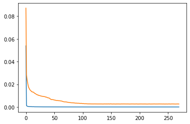
loss, mae, mse = model.evaluate(normed_test_data, test_labels, verbose=0)
print("Testing set Mean Abs Error: {:6.4f}".format(mae))
print("Testing set Mean Squared Error: {:6.4f}".format(mse))
1
2
Testing set Mean Abs Error: 0.0011
Testing set Mean Squared Error: 0.0002
1
2
3
4
# plot calculated metrics
plt.plot(history.history['mean_squared_error'])
plt.plot(history.history['mean_absolute_error'])
plt.show()

forex-prediction-results

The model can predict the closing price of the next bar with a MAE(mean absolute error) of 11 pips.
Cross validation will make the result more robust. A LSTM network would yield better results.