from __future__ import absolute_import, division, print_function, unicode_literals
import warnings
warnings.filterwarnings("ignore")
import pathlib
import matplotlib.pyplot as plt
import pandas as pd
import seaborn as sns
import tensorflow as tf
from tensorflow import keras
from tensorflow.keras import layers
print("Tensorflow Version : " + tf.__version__)
import sys
print("Python Version : " + sys.version)
from tensorflow.python.client import device_lib
print(device_lib.list_local_devices())
from sklearn import preprocessing
import numpy as np
from numpy.random import seed
import winsound
import os

checkpoint_path = "C:\\Users\\41507\\AppData\\Roaming\\MetaQuotes\\Terminal\\158904DFD898D640E9B813D10F9EB397\\MQL5\\Files\\ModelClose\\EURUSD\\modelClose.ckpt"
checkpoint_dir = os.path.dirname(checkpoint_path)

df = pd.read_csv('C:\\Users\\41507\\AppData\\Roaming\\MetaQuotes\\Terminal\\158904DFD898D640E9B813D10F9EB397\\MQL5\\Files\\EUR_USD_Test_H1.csv', header=0, delimiter=r"\s+")

print(df.shape)

df.columns = df.columns.str.replace("<", "")
df.columns = df.columns.str.replace(">", "")
# Extract date features
df['DATE'] = df['DATE'].astype('datetime64[ns]')
df['day_of_year'] = df['DATE'].dt.dayofyear
df['year'] = df['DATE'].dt.year

#Save Date in another dataframe for later use and then delete
dfDate = pd.DataFrame(df, columns=['DATE', 'TIME'])
del df['DATE']

df['TIME'] = df['TIME'].astype('datetime64[ns]')
df['hour_of_day'] = df['TIME'].dt.hour

#Save Time in another dataframe for later use and then delete
dfTime = pd.DataFrame(df, columns=['TIME'])
del df['TIME']

# Add column minmaxdiff
#df['score_diff'] = df['HIGH'].sub(df['LOW'], axis = 0)
#df['min_max_next'] = (df['HIGH']+df['LOW'])/2

# Add columns for previous candles
df['OPEN1'] = df['OPEN'].shift(1)
df['HIGH1'] = df['HIGH'].shift(1)
df['LOW1'] = df['LOW'].shift(1)
df['CLOSE1'] = df['CLOSE'].shift(1)
df['OPEN2'] = df['OPEN'].shift(2)
df['HIGH2'] = df['HIGH'].shift(2)
df['LOW2'] = df['LOW'].shift(2)
df['CLOSE2'] = df['CLOSE'].shift(2)
df['OPEN3'] = df['OPEN'].shift(3)
df['HIGH3'] = df['HIGH'].shift(3)
df['LOW3'] = df['LOW'].shift(3)
df['CLOSE3'] = df['CLOSE'].shift(3)
df['OPEN4'] = df['OPEN'].shift(4)
df['HIGH4'] = df['HIGH'].shift(4)
df['LOW4'] = df['LOW'].shift(4)
df['CLOSE4'] = df['CLOSE'].shift(4)
df['OPEN5'] = df['OPEN'].shift(5)
df['HIGH5'] = df['HIGH'].shift(5)
df['LOW5'] = df['LOW'].shift(5)
df['CLOSE5'] = df['CLOSE'].shift(6)
df['OPEN6'] = df['OPEN'].shift(6)
df['HIGH6'] = df['HIGH'].shift(6)
df['LOW6'] = df['LOW'].shift(6)
df['CLOSE6'] = df['CLOSE'].shift(6)
df['OPEN7'] = df['OPEN'].shift(7)
df['HIGH7'] = df['HIGH'].shift(7)
df['LOW7'] = df['LOW'].shift(7)
df['CLOSE7'] = df['CLOSE'].shift(7)
df['OPEN8'] = df['OPEN'].shift(8)
df['HIGH8'] = df['HIGH'].shift(8)
df['LOW8'] = df['LOW'].shift(8)
df['CLOSE8'] = df['CLOSE'].shift(8)
df['OPEN9'] = df['OPEN'].shift(9)
df['HIGH9'] = df['HIGH'].shift(9)
df['LOW9'] = df['LOW'].shift(9)
df['CLOSE9'] = df['CLOSE'].shift(9)
df.fillna(0, inplace=True)

step = -1
df['prediction_output'] = df['CLOSE'].shift(step)

n = 80
train_dataset = df.head(int(len(df)*(n/100)))
test_dataset = df.drop(train_dataset.index)
dfDate = dfDate.drop(train_dataset.index)

train_labels = train_dataset.pop('prediction_output')
test_labels = test_dataset.pop('prediction_output')
# Compare the shapes
print(train_labels.shape)
print(test_labels.shape)

def norm(x):
  return (x - train_stats['mean']) / train_stats['std']
normed_train_data = norm(train_dataset)
del normed_train_data['prediction_output']
normed_test_data = norm(test_dataset)
del normed_test_data['prediction_output']

def build_model():
  model = keras.Sequential([
    layers.Dense(64, activation=tf.nn.relu, input_shape=[len(normed_train_data.keys())]),
    layers.Dense(128, activation=tf.nn.relu),
    layers.Dense(128, activation=tf.nn.relu),
    layers.Dense(64, activation=tf.nn.relu),
    layers.Dense(1)
  ])

  optimizer = tf.keras.optimizers.RMSprop(learning_rate=0.003, rho=0.9)

  model.compile(loss='mean_squared_error',
                optimizer=optimizer,
                metrics=['mean_absolute_error', 'mean_squared_error'])
  return model

model = build_model()
model.summary()
# Display training progress by printing a single dot for each completed epoch
class PrintDot(keras.callbacks.Callback):
  def on_epoch_end(self, epoch, logs):
    if epoch % 100 == 0: print('')
    print('.', end='')

EPOCHS = 1000

# The patience parameter is the amount of epochs to check for improvement
early_stop = keras.callbacks.EarlyStopping(monitor='val_loss', patience=100)

# Create a callback that saves the model's weights
cp_callback = tf.keras.callbacks.ModelCheckpoint(filepath=checkpoint_path,
                                                 save_weights_only=True,
                                                 verbose=0)

history = model.fit(normed_train_data, train_labels, epochs=EPOCHS,
                    validation_split = 0.2, verbose=0, callbacks=[early_stop, PrintDot(), cp_callback])
hist = pd.DataFrame(history.history)
hist['epoch'] = history.epoch
hist.tail()

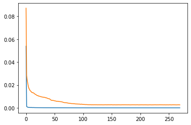
loss, mae, mse = model.evaluate(normed_test_data, test_labels, verbose=0)
print("Testing set Mean Abs Error: {:6.4f}".format(mae))
print("Testing set Mean Squared Error: {:6.4f}".format(mse))

# plot calculated metrics
plt.plot(history.history['mean_squared_error'])
plt.plot(history.history['mean_absolute_error'])
plt.show()